Naïve Bayes Algorithm in Machine Learning

Introduction to Naïve Bayes Algorithm in Machine Learning

The Naïve Bayes algorithm is a classification algorithm that is based on the Bayes Theorem, such that it assumes all the predictors are independent of each other. Basically, it is a probability-based machine learning classification algorithm which tends out to be highly sophisticated. It is very easy to build and can be used for large datasets.

Bayes Theorem:

Bayes theorem defines the likelihood of occurrence of an event that is based on some previous conditions related to that event. Or in simple words, it can be said that it is a way of calculating the Posterior probability from Likelihood, Class Prior Probability, and Predictor Prior Probability.

Mathematically;

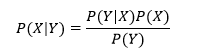
Where, is Posterior Probability, is a likelihood, is Class Prior Probability, and is Predictor Prior Probability from the equation given above.

As Bayes Theorem is a foundation of the Naïve Bayes machine learning algorithm, it requires some independence assumptions. So, the Naive Bayes machine learning algorithm often depends upon the assumptions which are incorrect. As we are working with the same dataset that we used in previous models, so in Bayes theorem, it is required age and salary to be an independent variable, which is a fundamental assumption of Bayes theorem.

But in our case, we can clearly see that fundamentally, it is not the case. There is some sort of correlation between them. As the person gets older, more the experience is gained, and simultaneously salary is increased. It can be seen that they are not absolutely independent. There is some sort of relation between the two variables.

Given that they are not independent, Bayes theorem can’t be applied to the machine learning algorithm. And this is the reason we apply Naïve Bayes to the machine learning algorithm. It is often applied at the time when the features and variables are not independent of each other. It is still applied and gives the best results.  

Types of Naïve Bayes Models

To build a Naïve Bayes model, the scikit learn library is used. There are three types of Naïve Bayes models that fall under the scikit learn python library, which is given below:

• Gaussian Naïve Bayes
• Multinomial Naïve Bayes
• Bernoulli Naïve Bayes

Gaussian Naïve Bayes model:

In this, the continuous feature values are considered assuming that the values of data are drawn from Gaussian distribution.

Multinomial Naïve Bayes model:

It is mostly used to classify document problems. The attributes are assumed to be drawn from a simple multinomial distribution. The model is best fitted for the attributes that denote discrete counts.

Bernoulli Naïve Bayes model:

It is mostly used in text classification problems. It assumes the features to be in a binary form (i.e., either 0 or 1). Only one value is taken up to forecast the class.

We will start by importing the python libraries.

.

1 2 3 4 5 6

# Importing the libraries import numpy as np import matplotlib.pyplot as plt import pandas as pd

After importing the libraries, we will then import the dataset and undergo pre-processing phase in the same way as we carried out in the earlier models.

1 2 3 4 5 6

# Importing the dataset dataset = pd.read_csv('Social_Network_Ads.csv') X = dataset.iloc[:, [2, 3]].values y = dataset.iloc[:, 4].values

1 2 3 4 5

# Splitting the dataset into the Training set and Test set from sklearn.model_selection import train_test_split X_train, X_test, y_train, y_test = train_test_split(X, y, test_size = 0.25, random_state = 0)

1 2 3 4 5 6 7

# Feature Scaling from sklearn.preprocessing import StandardScaler sc = StandardScaler() X_train = sc.fit_transform(X_train) X_test = sc.transform(X_test)

After pre-processing the data, we will fit the Naïve Bayes classifier to the training set. And for that, we will first import the GaussianNB class from scikit learn naïve bayes library, and then we will create its object naming it as a classifier. Here we do not need to input any parameter, we just need to call the class. We will then fit our classifier to the training set.  

1 2 3 4 5 6

# Fitting Naive Bayes to the Training set from sklearn.naive_bayes import GaussianNB classifier = GaussianNB() classifier.fit(X_train, y_train)

Since we have not passed any parameter in the above few lines, so we have GaussianNB in the output as shown below:

Output:

1 2 3

GaussianNB(priors=None, var_smoothing=1e-09)

Now that we are done fitting the classifier to the training set, we will now predict the test set results in the same manner as we did in the previous models. Basically, y_pred is the vector prediction containing all test set results. As we know, this is not a correct way to look at the incorrect predictions, and so we will construct a confusion matrix.

1 2 3 4 5 6 7

# Predicting the Test set results y_pred = classifier.predict(X_test) # Making the Confusion Matrix from sklearn.metrics import confusion_matrix cm = confusion_matrix(y_test, y_pred)

Output:

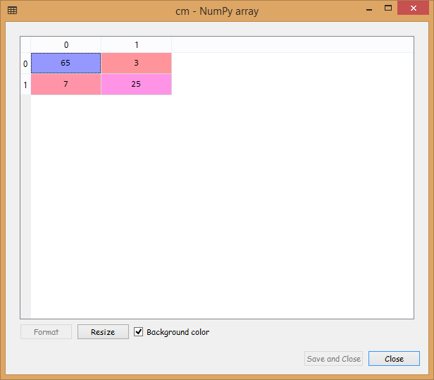
From the output image displayed above, it can be seen that we have 10 incorrect predictions out of 100.

Now we will get into the visualization part. In this step we will visualize both training set results as well as the test set results, by plotting a graph that will differentiate the region that predicts the users who will buy the SUV from the region predicting those users who will not but the SUV. It will be carried out in the same as we did in the earlier models.

1 2 3 4 5 6 7 8 9 10 11 12 13 14 15 16 17 18 19

# Visualising the Training set results from matplotlib.colors import ListedColormap X_set, y_set = X_train, y_train X1, X2 = np.meshgrid(np.arange(start = X_set[:, 0].min() - 1, stop = X_set[:, 0].max() + 1, step = 0.01),   np.arange(start = X_set[:, 1].min() - 1, stop = X_set[:, 1].max() + 1, step = 0.01)) plt.contourf(X1, X2, classifier.predict(np.array([X1.ravel(), X2.ravel()]).T).reshape(X1.shape),   alpha = 0.75, cmap = ListedColormap(('red', 'green'))) plt.xlim(X1.min(), X1.max()) plt.ylim(X2.min(), X2.max()) for i, j in enumerate(np.unique(y_set)):   plt.scatter(X_set[y_set == j, 0], X_set[y_set == j, 1],   c = ListedColormap(('red', 'green'))(i), label = j) plt.title('Naive Bayes (Training set)') plt.xlabel('Age') plt.ylabel('Estimated Salary') plt.legend() plt.show()

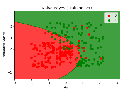
From the output image given above, it can be clearly seen that we have a very beautiful smooth curve with no irregularities. The naïve bayes model accomplished in gathering the older user with low estimated salary who bought the SUV in correct region, which was not classified correctly by the logistic regression and SVM model because of linearity. But in this case, the separator is a curve and it managed quite well to catch some of them.

1 2 3 4 5 6 7 8 9 10 11 12 13 14 15 16 17 18 19

# Visualising the Test set results from matplotlib.colors import ListedColormap X_set, y_set = X_test, y_test X1, X2 = np.meshgrid(np.arange(start = X_set[:, 0].min() - 1, stop = X_set[:, 0].max() + 1, step = 0.01),   np.arange(start = X_set[:, 1].min() - 1, stop = X_set[:, 1].max() + 1, step = 0.01)) plt.contourf(X1, X2, classifier.predict(np.array([X1.ravel(), X2.ravel()]).T).reshape(X1.shape),   alpha = 0.75, cmap = ListedColormap(('red', 'green'))) plt.xlim(X1.min(), X1.max()) plt.ylim(X2.min(), X2.max()) for i, j in enumerate(np.unique(y_set)):   plt.scatter(X_set[y_set == j, 0], X_set[y_set == j, 1],   c = ListedColormap(('red', 'green'))(i), label = j) plt.title('Naive Bayes (Test set)') plt.xlabel('Age') plt.ylabel('Estimated Salary') plt.legend() plt.show()

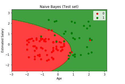
From the above image, we can clearly see the test set results. The naïve bayes classifier was successful in predicting most of the red users (who dint bought the SUV) in the red region as well as the green users (who bought the SUV) in the green region. We do have some incorrect predictions that are the red users in the green region or vice versa, and on counting them, it comes out to be 10, which is exactly equal to the incorrect predictions that we calculated in the confusion matrix in the earlier step. Since the results are the same and it ended up in classifying correctly, so we can say it is actually a good classifier. We will obtain some more shapes of the contour (prediction region) in the next models.

Advantages of Naïve Bayes Algorithm

1. It is the fastest algorithm and very easy to implement practically.
2. It performs better classification than the logistic regression model, as very little data is required for training.
3. It works well when the type of input data is categorical, but for numerical data, it presumes a normal distribution. 
4. Both discrete, as well as continuous data, can be handled by the Naïve Bayes algorithm.
5. It can be utilized for classification problems like binary and multiclass problems.

Disadvantages of Naïve Bayes Algorithm

1. Feature Independence: It is one of the biggest disadvantages of the algorithm, as it is next to impossible to have independent sets of features.
2. Zero Frequency: Suppose if a categorical variable has a specific category that is not witnessed in the training set, then, in that case, it will be assigned with a zero possibility that restricts it in making the prediction.

Applications of Naïve Bayes Algorithm

1. It can be used for real-time prediction.
2. It can be used for predicting multiple class variable’s posterior probabilities.
3. It is used for problems like text classification, filtering spam emails, and emotion analysis.